Measurement & Verification
Regression Analysis of Energy Saving Measures

Regression Analysis for Validation and Quantification of Energy Saving Measures
Version 2.2 - February 2019Trevor Boicey, P. Eng.
President, Ecovena
Purpose and Methodology
This document will explain how to use Linear Regression Analysis to validate and quantify the results of energy saving modifications to building heating systems.
Due to the variability of weather patterns, especially year-to-year differences, it is not possible to simply quantify energy usage patterns by consulting raw meter data, especially over smaller time periods.
To correct for weather variation, this analysis makes use of "Heating Degree Days", a correction factor that can be calculated from local weather history data. When factored into regression calculations, a building profile can be created that will predict, with significant accuracy, the energy required to maintain building temperature for any supplied weather condition.
Once a "before" profile is established, Energy Conservation Measures can be put in place, and allowed to run for a second measurement period, such as one complete heating season, to establish an "after" profile.
By comparing the "before" and "after" profiles, an accurate determination and quantification of the efficacy of the Energy Saving Measure can be obtained.
Data Gathering
Energy Consumption Data
Energy consumption data can be taken from any reliable source, such as a dedicated meter, a utility bill, or a series of spot measurements. In most cases, including in this document, utility consumption data is used. These values are assumed to be precise and are also available historically for defined time periods.
Heating Degree Days (HDD)
Basics of HDD
A single HDD value represents an amount of "heating requirement over time".
An HDD value can be assigned to a day, a month, or any arbitrary length of time. In most cases, HDD is calculated for each day, and the sum of all the HDD values for each day in a measurement period can be summed together. Typically the sums are made from all the dates to match a known energy measurement period, such as a utility billing interval.
As an example, an autumn day might have an HDD of 10. A week of the same weather would have an HDD of 7x10=70. And a 30 day month of identical weather would produce an HDD of 30x10=300.
Balance Point
All HDD calculations are based off of a chosen "balance point", which is expressed as a temperature. This temperature represents the threshold point, below which heat energy will be required to maintain building comfort, and above which no heat energy should be required.
Most calculations use one of two commonly used balance points, 15.5C and 18C. Note that these temperatures are slightly below the desired indoor temperatures, typically 21C. However, due to heat leakage from living activity (lights, appliances, cooking, body heat) most spaces maintain 21C even if the outdoor temperature is somewhat lower.
Calculations in this document use 15.5C as a balance point unless otherwise stated.
Computing HDD
A single day's HDD can be computed as follows:
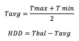
Example: An April day has a high temperature of 10C and a low temperature of 2C.

The HDD value for this April day is 6.
Note that HDD values are different if temperatures are stated in Fahrenheit or Celsius. All calculations in this document use Celsius.
Obtaining HDD data from Providers
In practice, many data providers supply HDD data as required, for any current or historical time period, with any balance point, ready to important into spreadsheets or other applications.
Data used in this document was supplied by BizEE Degree Days at https://www.degreedays.net/
Data Summing and Calculation
Calculations used in Regression Analysis are numerous but not complicated. For this document, we will be using a Microsoft Excel spreadsheet to perform the numerous sums and totals. The following screenshots show how the gathered data is arranged for calculation.


(these columns have one row per day for the entire measurement period of 2015-2018)


Regression Analysis
By plotting Energy Consumption on the Y-axis, and HDD for the same periods on the X-axis, a linear relationship is revealed.
Trendline Analysis
Using Excel, we add a linear trendline to the chart, and the software will also determine the linear equation formula for the derived line.
In the example "Pre" data, the formula for the trendline is:

Baseline Energy Usage
The intercept of the trendline with the Y-axis establishes the "Baseline Energy Usage". This represents the energy used by the building when supplemental heat is not required. As this data represents electricity usage, it comprises of energy used by non-heating circuits in the building, such as plugs, lights, elevators, etc.
The trendline has calculated the Baseline Energy Usage to be 60,314kW/h. This value should remain relatively consistent before and after Heating System Upgrades.
Weather Dependent Energy Usage
The x dependent term of the formula represents the increase in Energy Consumption by HDD. In the above example, consumption increases by 372.54 kW/h for every increment of one HDD. This is the term that will be improved by the Energy Saving Measure.
Importance of R2
The R2 term in the equation represents the "fit" of the data to the graph. High values of R2 allow high confidence in the derived data. A value of 1.0 indicates a perfect fit of all data to the trendline. A value above 0.95 represents a very good fit of data to the trendline. The example above of 0.99 represents data that can be used with a high level of confidence.
Pre and Post Energy Analysis
Validating R2 and Baseline Calculations
Referring again to the derived Pre and Post trendline equations:
For this data, the calculated baselines (60314 before, 60965 after) are within 1% of each other, representing strong data correlation.
Both R2 calculations, pre and post, are above 0.99, again, representing strong data correlation.
From these checks, it appears the data can be regarded as trustworthy.
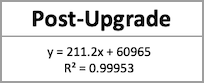
Comparing Pre and Post Trendline Slopes
The "pre" slope of 372.54 kW/h/HDD is significantly steeper than the "post" slope of 211.2kW/h/HDD.
By division, we can see that a temperature drop that would require 1kW/h more energy in the "pre" model, would only require 0.5669 kW/h more energy in the "post" model.
In other words, heat energy usage has been reduced by just over 43%.
Separating Heat Energy Usage from Baseline
With most utilities, energy consumed for heating is not 100% of the energy consumed. Electricity meter readings also include energy used for plugs and lights, while natural gas meter readings also include energy used for domestic hot water, laundry, etc.
To isolate heat energy usage over one year (12 months):
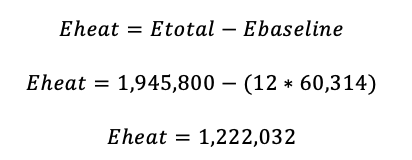
So the Total Energy Consumption was 1,945,800kW/h and the Heat Energy Consumption Portion was 1,222,032kW/h, or 62.8% of the total usage.
Expressing Heat Energy Savings as Percentage of Total Usage
For some purposes, it may be desired to represent the total energy savings as a percentage of the total energy consumption. Compensating for the fact that heat energy is only a portion of total consumption:

This energy saving measure saved 26.4% off the total Electrical Energy Consumption Bill.
Caveats
Daylight Variation
Due to differences in solar heating between high and low daylight months, some inaccuracies will be present when comparing some time periods. For highest accuracy, compare identical months between years when possible.
Human Activity Variation
Human behaviour will affect energy usage, and can repeat in cycles (weeks vs. weekends) or sporadically (statutory holidays, extreme weather).
For most properties, especially residential buildings, human behaviour can average out over longer time periods, such as one month or longer.
For more accurate data, measurement periods should be normalized to be the same length and to contain identical day patterns. (i.e.: the same number of weekdays vs. weekends)
For third party utility bills, this is often not possible, especially historically.
Cooling Expenses
Our analysis is primarily concerned with heating, and our geographic regions of interest have climates that have relatively low cooling energy requirements.
Specifically, our analysis generally covers building where cooling expenses are only significant for the two midsummer months of July and August, when window-mounted and temporary portable air conditioning units are in use.
To increase correlation (and to increase R2) it may be prudent to remove these months from any calculations. This will both improve R2 as well as the accuracy of the Baseline Energy Usage calculation.
Uncontrolled Variables
When comparing year-by-year data, it may require compensation for any other variations that may have occurred during these time periods. Example: Increasing efficiency of appliances, lighting upgrades, occupant turnover, etc.
When applying these calculations to a known building, it may be worthwhile to query present or past owners for any changes that may need to be accounted for.
Summary
In summation, the methods described here should be able to characterize building energy use for most structure, and to validate and quantify Energy Saving Measures over time.
For additional information on Energy Saving Measures in buildings, please contact Ecovena at http://www.ecovena.com/